Learning to Learn
How to Simulate

All the work done up to this point was compiled in the report and video linked below. Many improvements were added to the system since the last post. Due to time constraints, those changes are only described in the PDF below. Next steps will be to port the code to 3D, look into distributed training, and translate the model into C++ to create an interactive demo app using OpenGL. It might be interesting to look into creating a Houdini plugin for this at some point, but this will come later.

Here is the final report of my work done up to this point:

Here is a video of some results obtained with this simplified model to complement what's in my report:

TLDR: If you don't feel like reading the whole paper, but still have 18 minutes to spare, I have also recorded a high-level overview of this work embedded below.

Based on the results we've obtained in the last hyperparameter search we have identified that increasing the search radius for the graph creation allowed us to dramatically increase our ability to learn the global motion of the fluid. It turns out that PyTorch was a little bit misleading on this one… We were using a transformation called RadiusGraph to generate the graph on the GPU. This transform expects an argument called r. Believe it or not, r is not the search radius, but TWICE the search radius! Well of course!!!

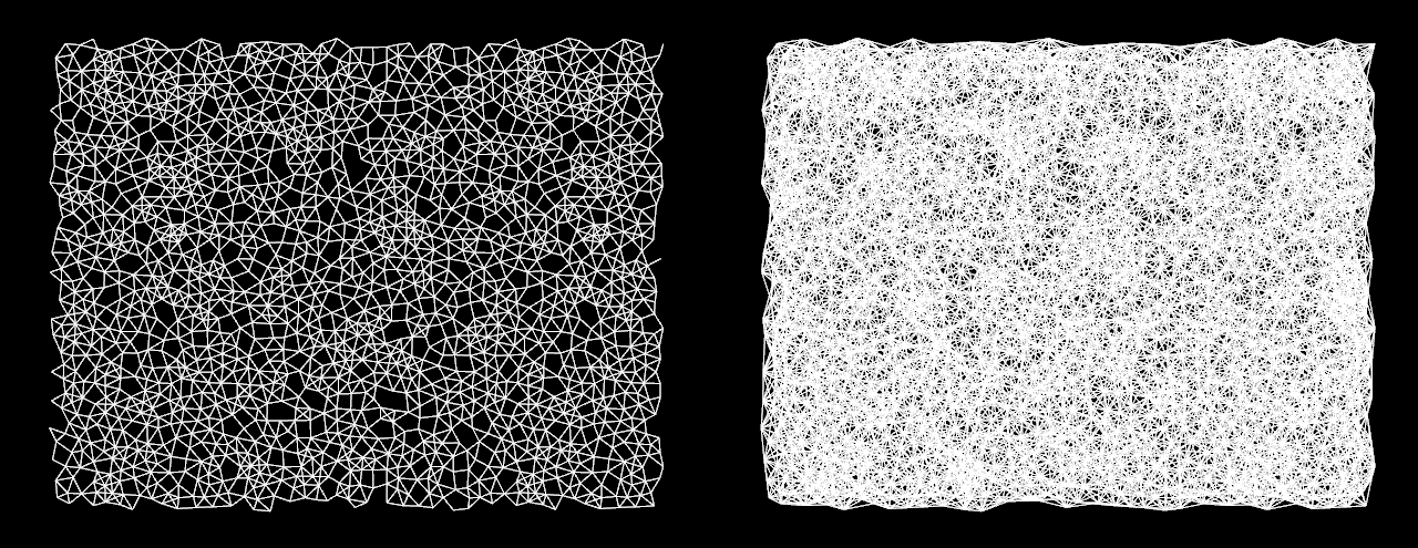
I figured this out when I built the graph in Houdini to compare it against the graph generated with PyTorch using a search radius of 0.015. Here is the result:

Doubling the search radius for the PyTorch graph (0.015 → 0.03) makes them match. It is important to make the graph denser than the one on the left since that one is missing a lot of neighbourhood information with such sparse connections.

Another important modification that we can do to our training loop is to schedule the learning rate to decay exponentially using the following formula.

$$ \eta \leftarrow \eta \left( \frac{1e-6}{1e-4} \right)^{\frac{1}{60000-20000}} $$

This can easily be translated into the following PyTorch code

    if batch_idx >= lr_decay_start and batch_idx < lr_decay_end:
        for g in optimizer.param_groups:
            g['lr'] *= lr_decay_step

where batch_idx is the gradient update step index and [lr_decay_start, lr_decay_end] is the range in which you want to decay the learning rate. In our case, lr_decay_start = 20000 and lr_decay_end = 60000.

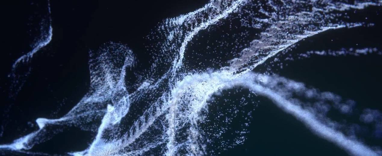
Using the scheduled learning rate described above as well as a search radius of 0.0125 (or 0.025 in PyTorch) we get the following results. Even though this is not there yet, this is very encouraging!

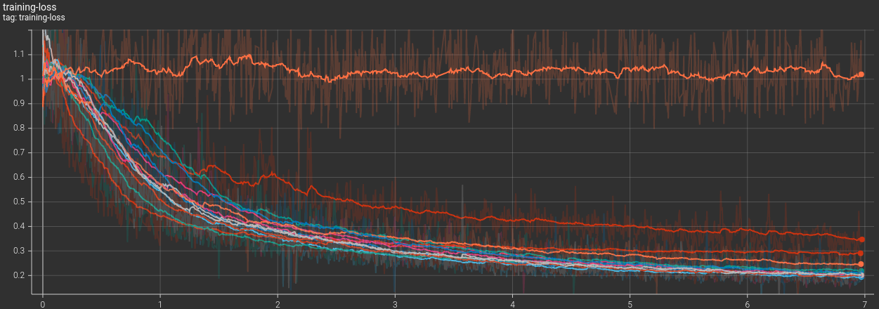
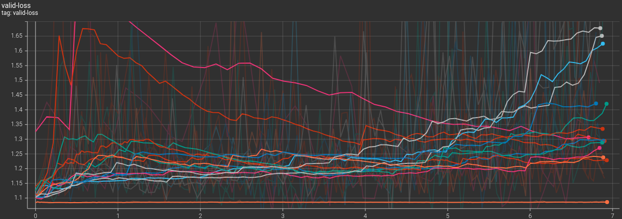
Before starting to implement more complex features in the model, it is a good idea to play a bit with the current architecture to see how different hyperparameters can influence how the model is able to learn the dynamics. Here we have performed 13 variations of our current model.

From looking at those graphs we may be tempted to draw some conclusions and do another pass of grid search, but we have to remember that at the moment we are using MSE as our loss function for both the single frame (training) and the full rollout (validation). Therefore, what might look fine or bad in MSE land may not translate into perceptual believability to a human looking at the sim. If you scroll down you can see the simulations that were generated by those 14 models trained for 7h each. By looking at the curves I would expect at least half of the models to perform similarly, but the results are very different from one model to the other. Even worse, the two models that perform best visually are not the ones with the best training and validation loss… A better metric like Earth-Mover will need to be used at some point.

After some time spent trying to properly understand the paper as well as the provided implementation I was able to write a first version of the model in PyTorch Geometric and train it for 12 hours on an Nvidia 1080 Ti.

In order to keep this first implementation as simple as possible multiple differences exist between the provided implementation from DeepMind and this one. As opposed to what the paper is doing, we are only providing the current velocity and position to the model instead of passing the 5 previous velocities. The idea is to allow the model to scale to bigger sims at some point. If we always require the 5 latest velocities to predict the next frame chances are that large simulations won't fit in GPU memory. Also, it feels like cheating when we know that traditional solvers do not require this information. The nodes and edges are encoded in a latent vector of size 64 as opposed to 128 in the paper. Again we want to see if we can compress the representation to save on memory. We are also not using the noise injection trick proposed in the paper to keep this first implementation as simple as possible. The particle type is not using an embedding of size 16. For now, we are only using a single integer to define the particle type. Our Adam optimizer is also using a learning rate of 0.0001 instead of the suggested exponential decay.

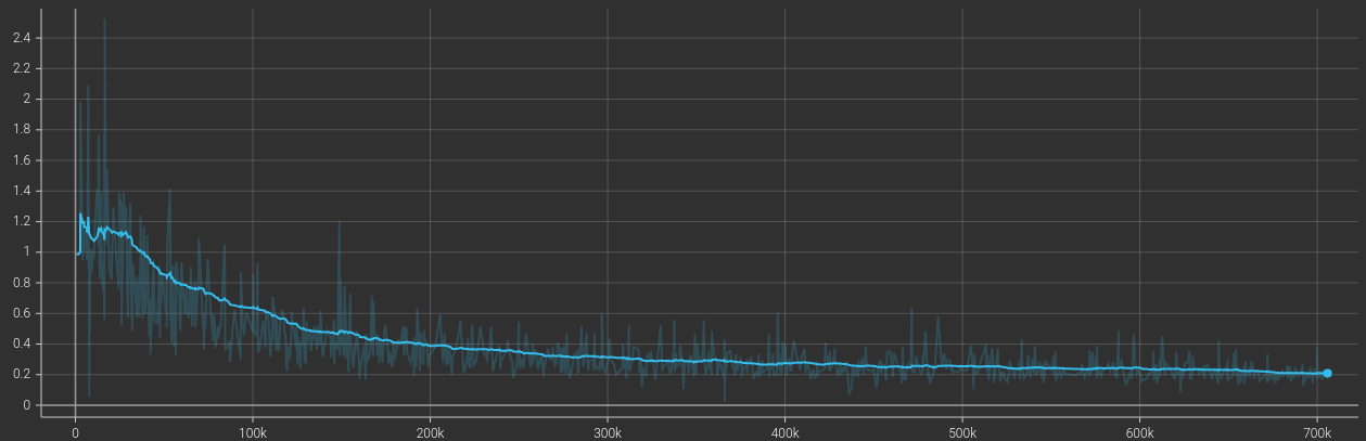
Here is the training curve we got for the 12h of training of this first implementation.

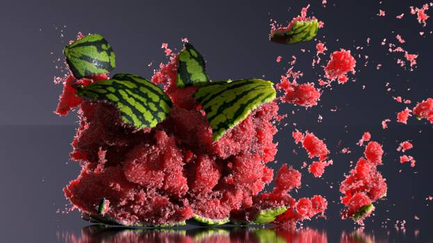
Here are the kind of animations we can get with this PyTorch implementation. It is definitely worse than the provided implementation, but at least it's a start and it shows that our implementation is not completely broken 👍.

In 2020, DeepMind released a paper about simulating multiple types of materials by training a Graph Network to replicate the results obtained with traditional particle solvers such as SPH, PBD and MPM.

Here is their original paper, along with the implementation they provide on GitHub based on Graph-Nets 1.1, TensorFlow 1.15 and Sonnet 1:

Here is a video of the results they obtained with their learned particle solver:

The results they obtained were very impressive in accuracy, but also fairly low-res compared to traditional methods. It seems like they have been focusing a lot more on the model's ability to generalize than the number of particles they could simulate or the training/inference speed they could reach.

Through the following posts, I will describe my attempts at re-implementing their work using PyTorch Geometric. The idea of changing of framework is to make sure I fully understand the implementation. It's too easy to be lazy and skip over the details when working in someone else's code. My goal is also to see if we can get inference time competitive to traditional particle solvers with this learned approach. I will also try to simplify the model in order to scale to bigger simulations if possible.